Lecture 4: Query Complexity of Boolean Functions
Date: February 13, 2026
- 1. Code Organization & Scope Management
- 2. (Finite) Subsets and Subtypes
- 3. Query Complexity of Boolean Functions
In this lecture we will formalize definitions in query complexity of Boolean functions (see the survey by Burhman and de Wolf). Our hope is that this will serve as a motivation for the kind of projects related to TCS that can be taken up in the course.
The main component of the lecture is covered in the demo. We will walk through this in the class, and fill in the gaps in the definitions and theorems there. The completed Lean source will be added here after the lecture.
In these lecture notes, we first touch upon additional key concepts in Lean not already covered that will be relevant for the demo. And then, we cover the relevant background on query complexity of Boolean functions as required for the demo.
1. Code Organization & Scope Management
We cover some common conventions for organizing code and managing scopes of variables.
variable
We can abstract away common arguments to def and theorem using variable.
For example, if we have (x : Nat) (h : x > 0) as binder for a sequence of
theorems, then we can define it once using variable and it gets introduced
for each theorem in the group.
Note: Lean automatically inserts the variable as an argument only if the definition actually uses it.
variable (α : Type)

def myId (a : α) : α := a

#check myId   -- Output: myId (α : Type) (a : α) : α
namespace
namespace allows logical grouping with name prefixing.
This allows us to avoid name collisions (e.g., distinguishing Nat.add from
Int.add), by automatically prepending the namespace name to every definition
inside.
Note: Variables/definitions created inside remain associated with that namespace.
namespace MySpace

  -- Full name: MySpace.foo
  def foo : Nat := 10

  -- Full name: MySpace.bar
  -- Can call 'foo' directly here because we are inside the namespace
  def bar : Nat := foo + 5

end MySpace

-- Outside, must use full name
#check MySpace.foo
section
section allows limiting the scope of variable commands (and also open
commands, discussed next). But crucially, unlike namespace, it does not
change the name of definitions. So section is useful for setting up common
parameters (hypotheses) for a block of theorems, and then discarding them.
Syntax:
section MySection

  variable (n : Nat) -- 'n' is now an argument for everything in this section

  def double : Nat := n + n

end MySection
-- 'n' is no longer a set variable here

#check double  -- Name is just 'double', NOT 'MySection.double'
open
open allows for accessing names without the namespace prefixes. In the above
example, this allows writing foo instead of MySpace.foo.
Once open is applied, it applies to the current “block”, that is, until the
end of namespace or section, or simply end of file.
open can be applied in three variants:
Standard open:
Opens for the remainder of the current scope.
open List
#check map  -- Works (refers to List.map)
Scoped open (inside Section):
Demonstrates how section acts as a container for open.
section
  open List
  -- 'map' works here (refers to List.map)
end
-- 'map' no longer works here; the section closed the scope.
Inline open ... in:
Opens a namespace only for the execution of the immediately following command.
-- Opens 'List' just for this definition
open List in
def myFunc : List Nat := map (· + 1) [1, 2, 3]
2. (Finite) Subsets and Subtypes
In Lean, every element has a unique type. So if we want to index over natural numbers in $\{0, \ldots, n-1\}$, then we would need to create a new type for it.
Such a type can be created as {x : Nat // x < 5}. More generally subtypes of α can be created as { x : α // p x} (or simply { x // p x}, since the type of x can be inferred).
An element of a subtype is a structure with a value (val) and a proof (property) that val satisfies the said property.
def x : {z : ℕ // z < 5} := ⟨3, by simp⟩

-- You access the value using .val or .1, or prefixing by ↑.
#check x.val -- This is a Nat (3)
#check x.property -- This is a proof (3 < 5)
#eval ↑x          -- Same as x.val
A subtype is distinct from a set, which would be defined as {x : Nat | x < 5}.
Notes will be added on Fin, Finset and Fintype shortly.
3. Query Complexity of Boolean Functions
We consider two complexity measures of Boolean functions $f : \{0, 1\}^n \to \{0, 1\}$.
Decision Tree Complexity
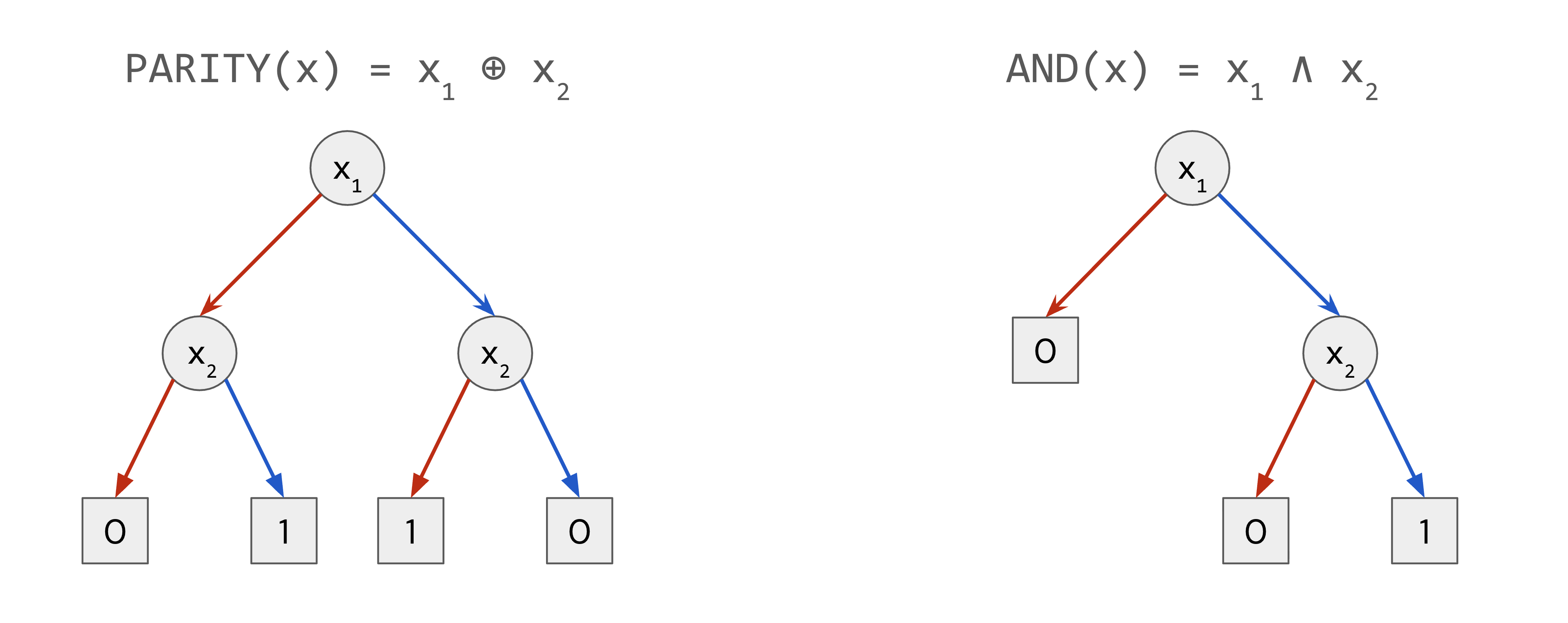
A decision tree is a binary tree where every internal node is labeled with an index $i \in [n]$ and every leaf is labeled with a value in $\{0, 1\}$.
A decision tree evaluates an input $x \in \{0, 1\}^n$ by starting at the root, and recursively querying the variable at the index specified by the node. If the variable is $0$, the algorithm moves to the left branch, and if the variable is $1$, it moves to the right branch. Once at a leaf, the corresponding value is returned.
Below are examples of decision trees that compute the two bit Parity function and the two-bit And function.
For any Boolean function $f : \{0, 1\}^n \to \{0, 1\}$, its decision tree complexity $D(f)$ is the smallest depth of a decision tree that computes $f$.
Sensitivity
The sensitivity of a Boolean function $f : \{0, 1\}^n \to \{0, 1\}$ at input $x \in \{0, 1 \}^n$ is $s(f, x) := |\{ i : f(x) \ne f(x^{\oplus i})\}|$, the number of coordinates of $x$ that when flipped, change the value of the function $f$.
The sensitivity of $f$ is $s(f) := \max_{x \in \{0, 1\}^n} \ s(f, x)$.
Theorem: Sensitivity ≤ Decision Tree Complexity
The main theorem we will work through in this lecture is the following:
Theorem. For all $f : \{0, 1\}^n \to \{0, 1\}$ : $s(f) \leq D(f)$.
Proof Sketch.
Consider a decision tree $T$ that computes $f$. On any input
$x \in \{0, 1\}^n$, if the decision tree $T$ does not query a sensitive bit
$i \in [n]$ of $x$, then it might compute either $f(x)$ or $f(x^{\oplus i})$
incorrectly.
$\square$
See demo for the Lean file to work through these definitions and proofs.
Further Topics
Query Complexity of Boolean functions is a rich research topic. There are numerous other complexity measures of which we name a few:
- Randomized Query Complexity (Bounded-error, Unbounded-error, One-sided error, Zero error)
- Quantum Query Complexity
- Block sensitivity
- Degree, Approximate degree, Threshold degree, Rational degree
New breakthroughs continue to happen even in the last few years, some notable examples being the proof of the Sensitivity Conjecture, and a more recently the Rational Degree Conjecture.
Formalizing old / new results in this area could be a ripe topic for course projects!